| Product-Name |
Butybond AB15 |
Solabond FS15 |
Solabond FSP18 |
Solabond FS18 |
Solabond PSP15 |
Thermobond STP18 |
Thermobond QTP18 |
Thermobond RT21 |
| General Description |
|
|
|
|
|
|
|
|
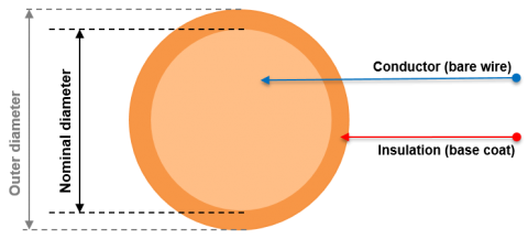
| Base coat |
mod. Polyurethane |
mod. Polyurethane |
mod. Polyurethane |
Polyesterimide |
mod. Polyurethane |
mod. Polyurethane |
mod. Polyurethane |
A200 + Polyamidimide |
| Bond coat |
Polyvinylbutyral |
Polyamide |
Polyamide |
Polyamide |
Polyamide |
Polyamide |
Polyamide |
aromatic Polyamide |
| IEC (including the following standards) |
IEC 60317-35, 60317-2 |
IEC 60317-35, 60317-2 |
|
IEC 60317-36 |
IEC 60317-35, 60317-2 |
|
IEC 60317-35 |
IEC 60317-38 |
| NEMA (including the following standards) |
MW 131-C |
MW 131 |
|
|
MW 131 |
MW 131 |
MW 131 |
MW 102 |
| Diameters available |
0.01 - 0.50 mm |
0.01 - 0.50 mm |
0.01 - 0.50 mm |
0.01 - 0.50 mm |
0.01 - 0.50 mm |
0.01 - 0.50 mm |
0.015 - 0.50 mm |
0.015 - 0.50 mm |
| Properties |
Low bonding temperature, wide process window, non-hygroscopic |
All bonding methods applicable, good processability, hygroscopic (not suited for humid regions) |
All bonding methods applicable, good processability, hygroscopic |
Solvent bonding possible, high resoftening temperature, high thermal and mechanical properties of base coat, hygroscopic thus not suitable for Asia |
All purpose selfbonding enamel, wide process window, high bonding strength, thermosetting applicable, non-hygroscopic |
Good winding ability, thermosetting applicable |
higher thermal and mechanical properties, very high resoftening temperature after thermosetting |
very high thermal and mechanical properties, very high resoftening temperature |
Shelf life in months (at 25°C /
60% rel. humidity) |
≤ 6 |
≤ 3 (hygroscopic) |
≤ 5 (hygroscopic) |
≤ 5 (hygroscopic) |
≤ 6 |
≤ 6 |
≤ 6 |
≤ 6 |
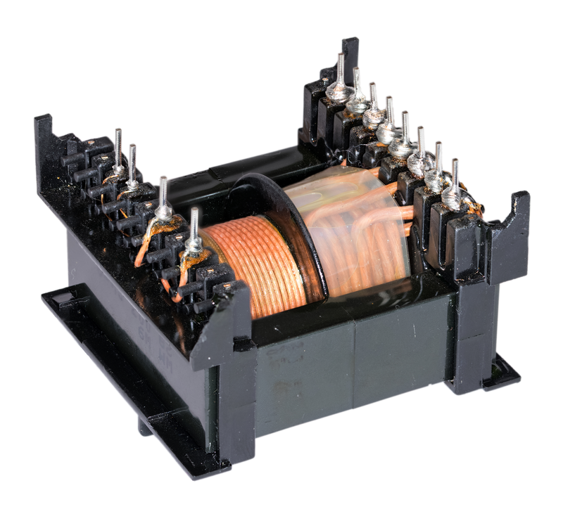
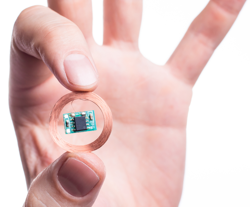
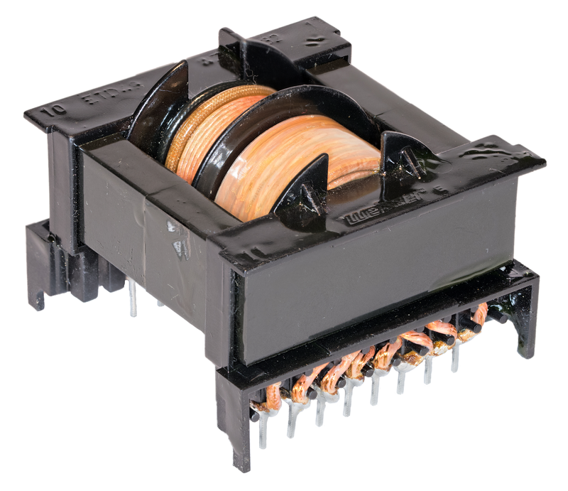
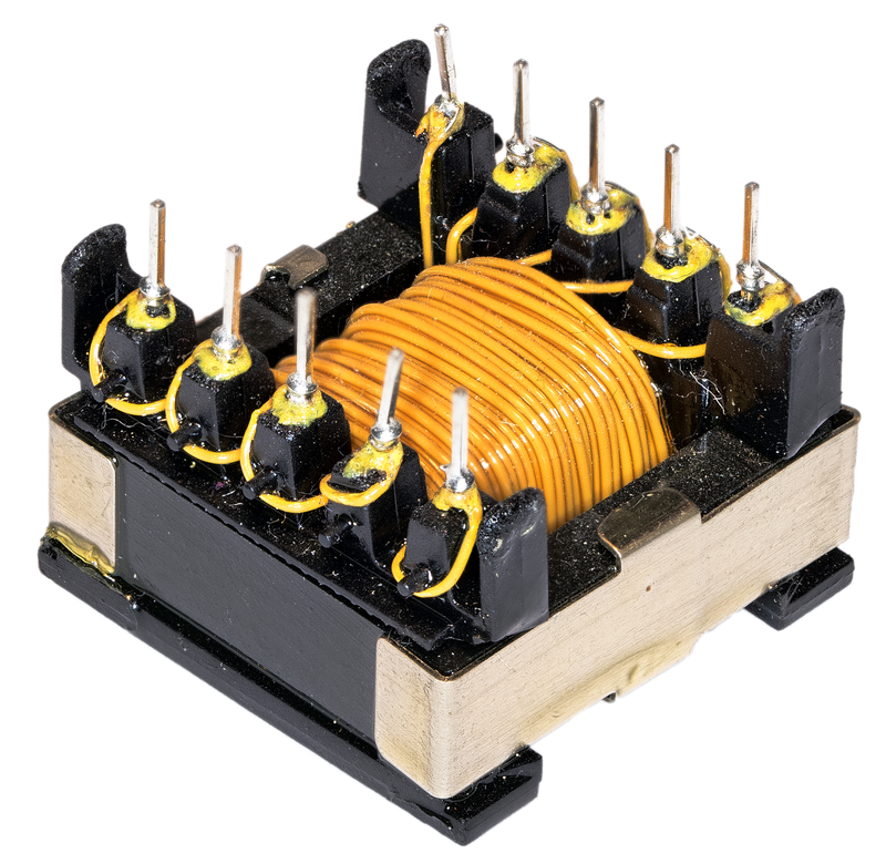
| Applications |
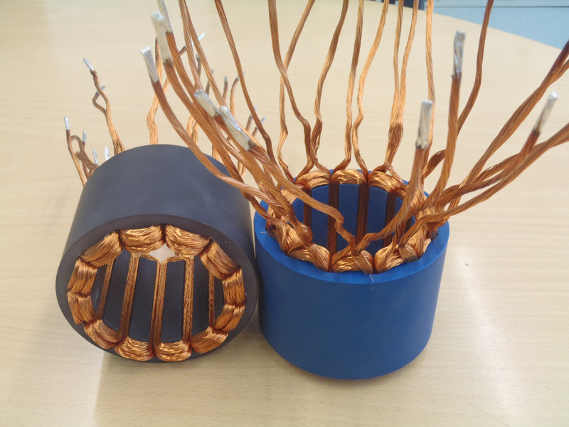
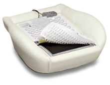
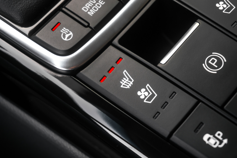
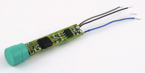
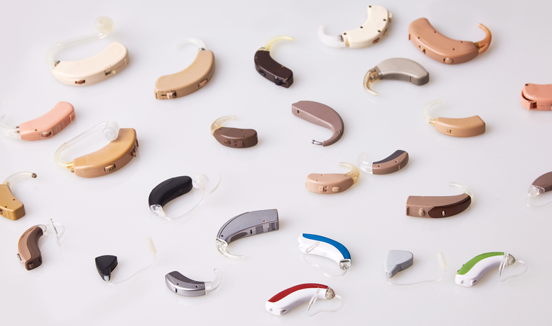
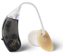
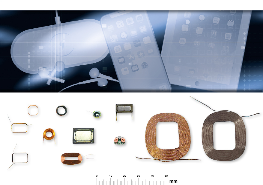
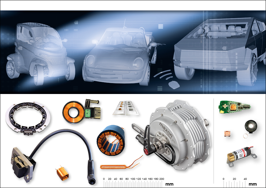
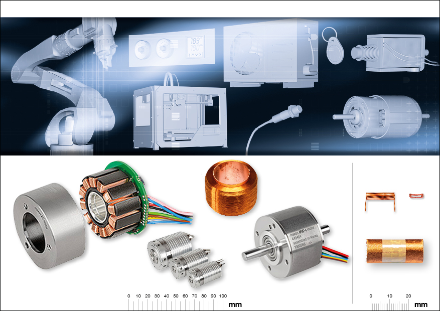
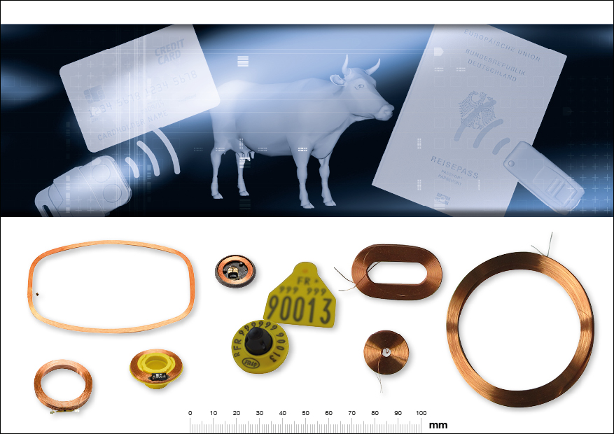
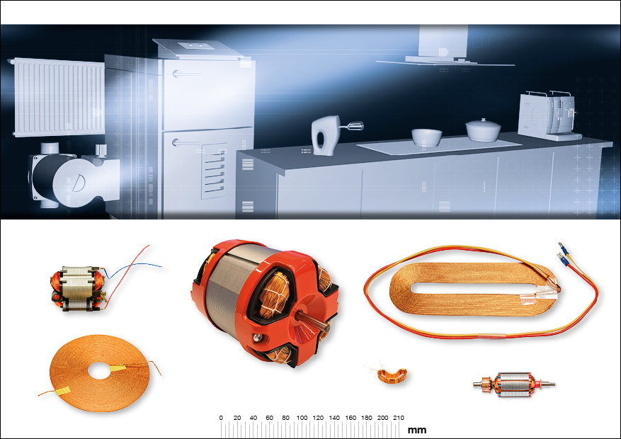
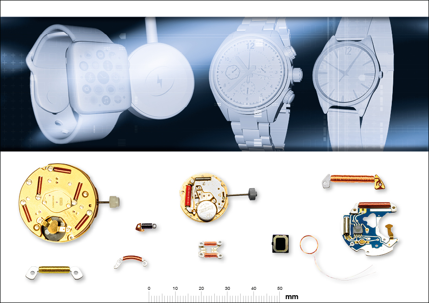
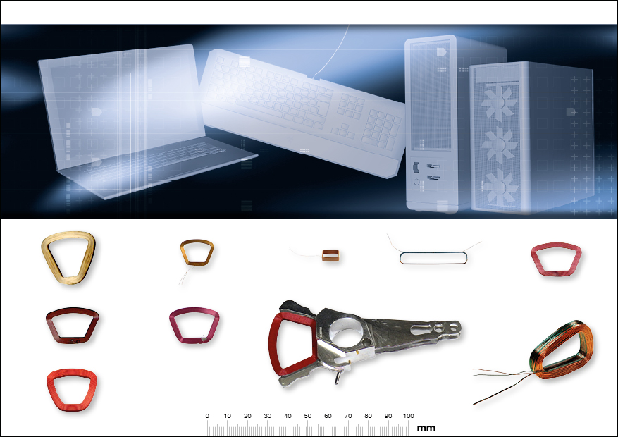
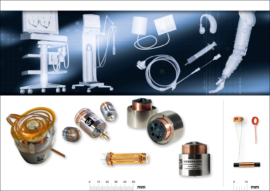
Stepping motors for quartz watches, instrument coils, voice coils, Sensors, Transponders |
Loudspeakers, small motors, sensors, Transponders |
Loudspeakers, small motors, sensors, Transponders |
Loudspeakers, small motors, sensors, Transponders |
Instrument coils, loudspeakers, vibration motors, sensors, receiver and speaker for mobile phones |
High power speaker, vibration motors |
high power speaker and receiver, micro speaker, high temperature applications |
motors, loudspeakers |
| Thermal values of base coat |
|
|
|
|
|
|
|
|
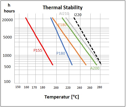
| Temperature index 20.000 h acc. to IEC 60172 |
158°C |
158°C |
192°C |
195°C |
158°C |
192°C |
192°C |
212°C |
|
Thermal stability chart [view]
|
|
|
|
|
|
|
|
|
| Cut through temperature |
|
|
|
|
|
|
|
|
| 0.05mm: acc. to IEC 60851-6 4 |
≥ 200°C |
≥ 200°C |
≥ 230°C |
≥ 265°C |
≥ 200°C |
≥ 230°C |
≥ 230°C |
≥ 320°C |
| Elektrisola typical value |
225°C |
225°C |
260°C |
315°C |
225°C |
260°C |
260°C |
365°C |
| 0.25mm: acc. to IEC 60851-6 4 |
≥ 200°C |
≥ 200°C |
≥ 230°C |
≥ 265°C |
≥ 200°C |
≥ 230°C |
≥ 230°C |
≥ 320°C |
| Elektrisola typical value |
230°C |
230°C |
265°C |
325°C |
230°C |
265°C |
265°C |
380°C |
| Heat Shock |
|
|
|
|
|
|
|
|
| 0.05mm: acc. to IEC 60851-6 3 |
≥ 175°C |
≥ 175°C |
≥ 200°C |
≥ 200°C |
≥ 175°C |
≥ 200°C |
≥ 200°C |
≥ 220°C |
| Elektrisola typical value |
190°C |
190°C |
210°C |
260°C |
190°C |
210°C |
210°C |
250°C |
| 0.25mm: acc. to IEC 60851-6 3 |
≥ 175°C |
≥ 175°C |
≥ 200°C |
≥ 200°C |
≥ 175°C |
≥ 200°C |
≥ 200°C |
≥ 220°C |
| Elektrisola typical value |
180°C |
180°C |
200°C |
250°C |
180°C |
200°C |
200°C |
240°C |
| Electrical values |
|
|
|
|
|
|
|
|
| Low voltage continuity for Grade 1B wires |
|
|
|
|
|
|
|
|
| 0.05mm: acc. to IEC 60851-5 1 |
≤ 40 |
≤ 40 |
≤ 40 |
≤ 40 |
≤ 40 |
≤ 40 |
≤ 40 |
≤ 40 |
| Elektrisola typical value |
0 |
0 |
0 |
0 |
0 |
0 |
0 |
0 |
| High voltage continuity for Grade 1B wires |
|
|
|
|
|
|
|
|
| 0.05mm: Elektrisola typical value |
0 |
0 |
0 |
0 |
0 |
0 |
0 |
0 |
| 0.25mm: acc. to IEC 60851-5 2 |
≤ 10 |
≤ 10 |
≤ 10 |
≤ 10 |
≤ 10 |
≤ 10 |
≤ 10 |
≤ 10 |
| 0.25mm: Elektrisola typical value |
0 |
0 |
0 |
0 |
0 |
0 |
0 |
0 |
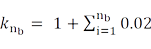
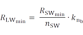
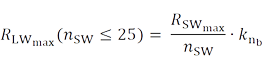
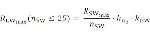
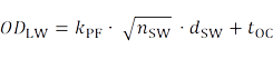
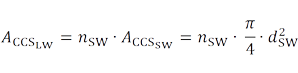
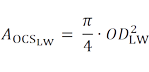
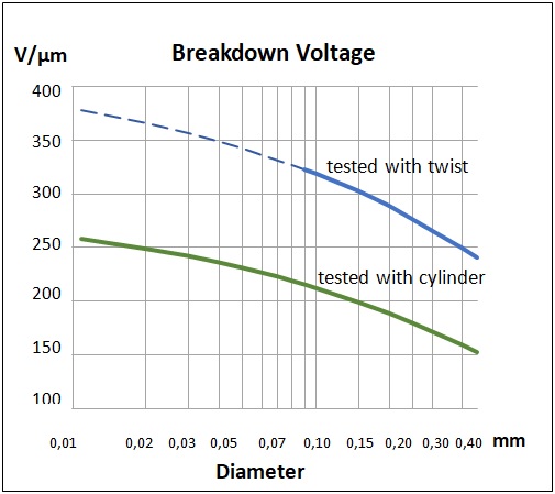
| Breakdown voltage acc. to IEC 60851-5 4 (at 20 °C, 35% humidity) |
|
|
|
|
|
|
|
|
| 0.05mm: Elektrisola typical value |
160 V/µm |
160 V/µm |
160 V/µm |
160 V/µm |
160 V/µm |
160 V/µm |
160 V/µm |
160 V/µm |
| 0.25mm: Elektrisola typical value |
120 V/µm |
120 V/µm |
120 V/µm |
120 V/µm |
120 V/µm |
120 V/µm |
120 V/µm |
120 V/µm |
|
Calculation method of break voltage [view]
|
|
|
|
|
|
|
|
|
| Pinholes acc. to IEC 60851-5 7 |
|
|
|
|
|
|
|
|
| 0.05mm: with 0% elongation |
good |
good |
very good |
very good |
very good |
very good |
|
|
| 0.25mm: with 0% elongation |
good |
good |
very good |
very good |
very good |
very good |
|
|
| Mechanical values |
|
|
|
|
|
|
|
|
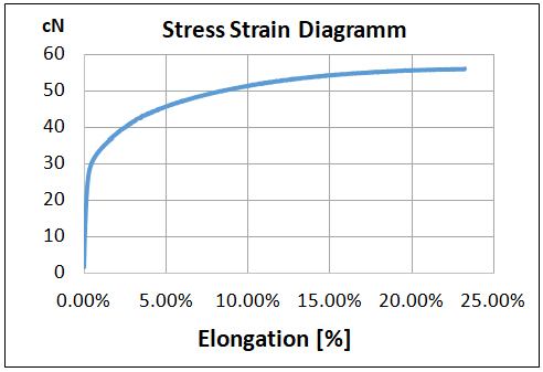
| Elongation for Grade 1B wire |
|
|
|
|
|
|
|
|
| 0.05mm: acc. to IEC 60851-3 3.1 |
≥ 14% |
≥ 14% |
≥ 14% |
≥ 14% |
≥ 14% |
≥ 14% |
≥ 14% |
≥ 14% |
| Elektrisola typical value |
23% |
23% |
23% |
23% |
23% |
23% |
23% |
23% |
| 0.25mm: acc. to IEC 60851-3 3.1 |
≥ 25% |
≥ 25% |
≥ 25% |
≥ 25% |
≥ 25% |
≥ 25% |
≥ 25% |
≥ 25% |
| Elektrisola typical value |
40% |
40% |
40% |
40% |
40% |
40% |
40% |
40% |
| Tensile strength for Grade 1B wires |
|
|
|
|
|
|
|
|
| 0.05mm: Elektrisola typical value |
57 cN |
57 cN |
57 cN |
57 cN |
57 cN |
57 cN |
57 cN |
57 cN |
| 0.25mm: Elektrisola typical value |
1370 cN |
1370 cN |
1370 cN |
1370 cN |
1370 cN |
1370 cN |
1370 cN |
1370 cN |
|
Stress strain chart [view]
|
|
|
|
|
|
|
|
|
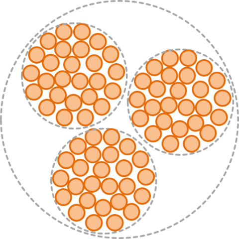
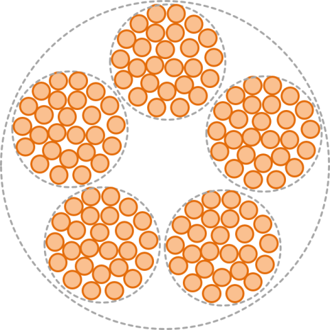
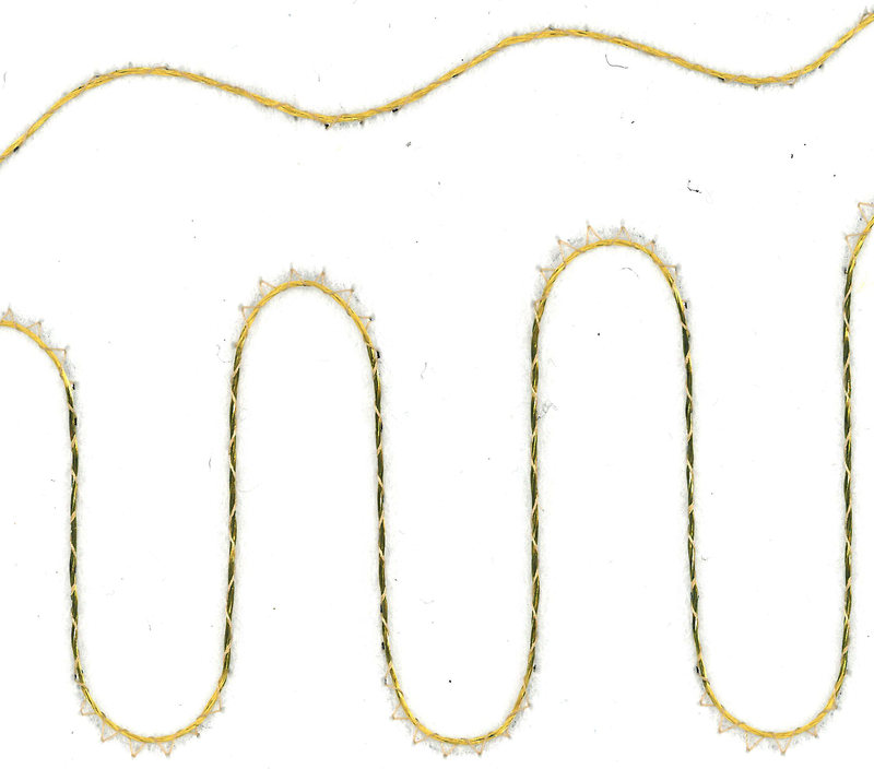
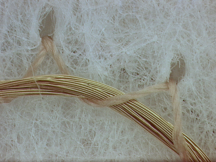
| Bonding of wire |
|
|
|
|
|
|
|
|
| Hot air bonding |
0.01 - 0.50 mm |
0.01 - 0.50 mm |
0.015 - 0.50 mm |
0.01 - 0.50 mm |
0.01 - 0.50 mm |
0.01 - 0.50 mm |
0.015 – 0.50 mm |
limited |
| Oven bonding |
0.10 - 0.50 mm |
0.10 - 0.50 mm |
0.10 - 0.50 mm |
0.10 - 0.50 mm |
0.10 - 0.50 mm |
0.10 - 0.50 mm |
0.10 – 0.50 mm |
0.10 – 0.50 mm |
| Resistance bonding |
0.10 - 0.50 mm |
0.10 - 0.50 mm |
0.10 - 0.50 mm |
0.10 - 0.50 mm |
0.10 - 0.50 mm |
0.10 - 0.50 mm |
0.10 – 0.50 mm |
0.10 – 0.50 mm |
| Solvent bonding |
limited |
suitable |
suitable |
suitable |
not suitable |
not suitable |
not suitable |
not suitable |
| Recommended solvent |
Ethanol / Methanol |
Ethanol / Methanol |
Ethanol / Methanol |
Ethanol / Methanol |
N/A |
N/A |
N/A |
N/A |
| Recommended bonding temperature |
120 - 140°C |
150 - 170°C |
150 - 170°C |
150 - 170°C |
150 - 170°C |
180 - 200°C |
200 – 220°C |
200 – 220°C |
Resoftening temperature for 0.25mm
(IEC 60851-3 7.1.2.4) |
≥ 100°C |
≥ 140°C |
≥ 170°C |
≥ 180°C |
≥ 180°C |
≥ 145°C |
≥ 190°C |
≥ 200°C |
| Bond strength chart |
|
|
|
|
|
|
|
|
| RoHS laboratory analysis |
view |
view |
view |
view |
|
view |
|
|
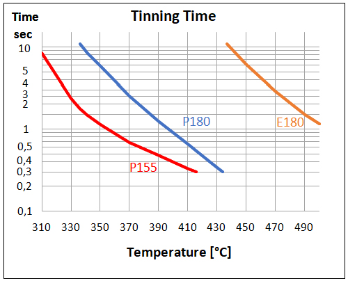
| Solderability |
|
|
|
|
|
|
|
|
| Solderability for Grade 1B wires |
|
|
|
|
|
|
|
|
| 0.05mm: max. acc. to IEC 60851-4 5 |
2.0s / 390°C |
2.0s / 390°C |
2.0s / 390°C |
3.0s / 470°C |
2.0s / 390°C |
3.0s / 390°C |
3.0s / 390°C |
--- |
| Elektrisola typical value |
0.8s / 390°C |
0.4s / 390°C |
0.7s / 390°C |
1.3s / 470°C |
0.4s / 390°C |
0.4s / 420°C |
1.0s / 390°C |
--- |
| Elektrisola typical value |
1.5s / 370°C |
0.5s / 370°C |
1.0s / 370°C |
|
0.7s / 370°C |
--- |
|
|
| 0.25mm: max. acc. to IEC 60851-4 5 |
3.0s / 390°C |
3.0s / 390°C |
3.0s / 390°C |
3.0s / 470°C |
3.0s / 390°C |
3.0s / 390°C |
3.0s / 390°C |
--- |
| Elektrisola typical value |
1.4s / 390°C |
0.7s / 390°C |
1.6s / 390°C |
3.0s / 470°C |
0.7s / 390°C |
0.8s / 420°C |
2.0s / 390°C |
--- |
| Elektrisola typical value |
2.0s / 370°C |
1.2s / 370°C |
2.8s / 370°C |
|
1.2s / 370°C |
|
|
|
|
Solderability of different wire types chart [view]
|
|
|
|
|
|
|
|
|


